通过 MATLAB 实现基本的单变量线性回归，并绘制梯度图。

这是本学期我的 ML 实验报告。实验报告的题目为 Andrew Ng (吴恩达) 的 Stanford Machine Learning 课程。实验报告编号可能与课程页面的编号略有差别，但问题不大。

# Experiment 1: Linear Regression

This is the report of Experiment 1: Linear Regression.

# Purpose

In this experiment, we have the data of ages and heights. We want to find the connection of these two groups of data.

# Hypothesis

We hypothesize that ages($x$) and heights($y$) are linear dependent.

# Procedure and Results

We implement linear regression using gradient decent. The gradient decent update rule is

$$\theta_j = \theta_j - \alpha\frac{1}{m}\sum_{i=1}^m\left(h_{\theta}(x^{(i)}) - y^{(i)}\right)x^{(i)}_j, \quad j = 0,1$$

We let learning rate $\alpha = 0.07$.

After the first iteration, we got the value of theta is

$$\theta_0 = 0.00686133, \quad \theta_1 = 0.15017321$$

After $1500$ iterations, the value of data is

$$\theta_0 = 0.03750784, \quad \theta_1 = 0.10655703$$

The figure of the result is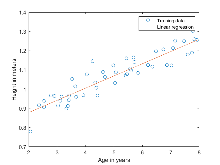

Using the model, we can know that while the age is $3.5$, the height is

$$\hat{h}(3.5) = \theta_0 + 3.5\theta_1 = 0.97322864$$

When the age is $7$, the height is

$$\hat{h}(7) = \theta_0 + 7\theta_1 = 1.19584369$$

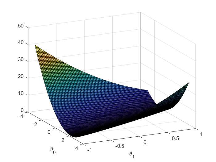
Then, I draw the figure to visualize the relationship between $\theta_0$ and $\theta_1$, let

$$J(\theta_0, \theta_1) := \frac{1}{2m}\sum_{i=1}^m(h_\theta(x^{(i)})-y^{(i)})^2$$

The figure is as follow: